目录
一、说明
二、初步:多元高斯分布
三、 线性回归模型与维度的诅咒
四、高斯过程的数学背景
五、高斯过程的应用:高斯过程回归
5.1 如何拟合和推理高斯过程模型
5.2 示例:一维数据的高斯过程模型
5.3 示例:多维数据的高斯过程模型
六、引用

照片由 理查德·霍瓦特 on Unsplash
一、说明
G澳大利亚的过程是有益的,特别是当我们有少量数据时。当我在制造业担任数据科学家时,我们的团队使用这种算法来揭示我们接下来应该进行哪些实验条件。但是,此算法不如其他算法流行。在这篇博客中,我将通过可视化和 Python 实现来解释高斯过程 [1] 的数学背景。
二、初步:多元高斯分布
多元高斯分布是理解高斯过程的必要概念之一。让我们快速回顾一下。如果您熟悉多元高斯分布,则可以跳过此部分。
多元高斯分布是具有两个以上维度的高斯分布的联合概率。多元高斯分布的概率密度函数如下。

多元高斯分布的概率密度函数
x 是具有 D × 1 维的输入数据,μ 是与 x 具有相同维数的平均向量,Σ 是具有 D × D 维的协方差矩阵。
多元高斯分布具有以下重要特征。
- 多元高斯分布的边际分布仍然遵循高斯分布
- 多元高斯分布的条件分布仍然遵循高斯分布
让我们通过可视化来检查这些概念。我们假设 D 维数据服从高斯分布。
对于特征 1,当我们将输入数据维数 D 划分为第一个 L 和其他 D-L=M 维时,我们可以将高斯分布描述如下。

分离多元高斯分布
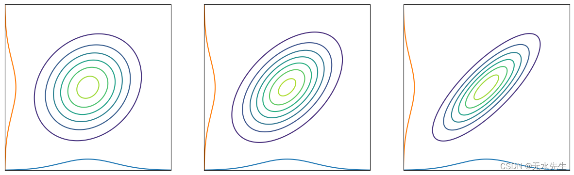
然后,当我们边缘化 x₂ 的分布时,x₁ 的概率分布可以写成:
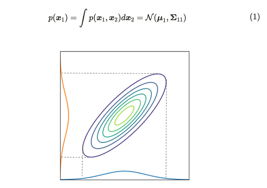
二维高斯分布的边际分布
根据公式(1),我们可以在边缘化其他变量时取消它们。该图显示了二维高斯分布情况。正如你所看到的,边缘化的分布映射到每个轴;它的形式是高斯分布。直观地说,当我们根据一个轴切割多元高斯分布时,横截面的分布仍然遵循高斯分布。您可以查看参考文献 [2] 以获取详细推导。
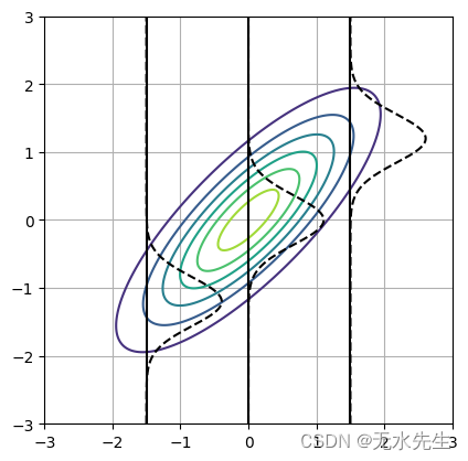
对于特征 2,我们使用相同的 D 维多元高斯分布和二分输入数据 x₁ 和 x₂。多元高斯分布的条件概率可以写成:
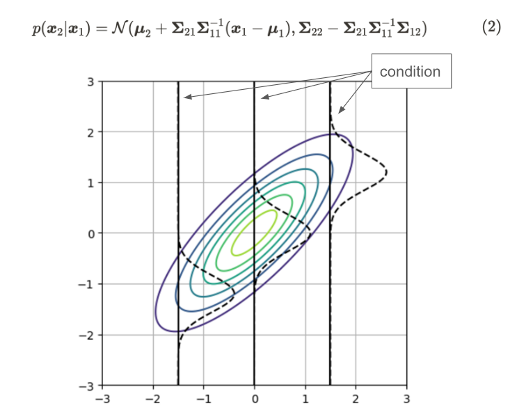
二维高斯分布的条件分布
该图显示了二维高斯分布(等值线)和条件高斯分布(虚线)。高斯分布的形状在每种条件下都不同。您可以查看参考文献 [2] 以获取详细推导。
三、 线性回归模型与维度的诅咒
在深入研究高斯过程之前,我想澄清线性回归模型及其缺点或维数的诅咒。高斯过程与这个概念密切相关,可以克服其缺点。如果本章响起,您可以跳过本章。
让我们回顾一下线性回归模型。线性回归模型可以使用基函数 φ(x) 灵活地表达数据。

线性回归模型的公式
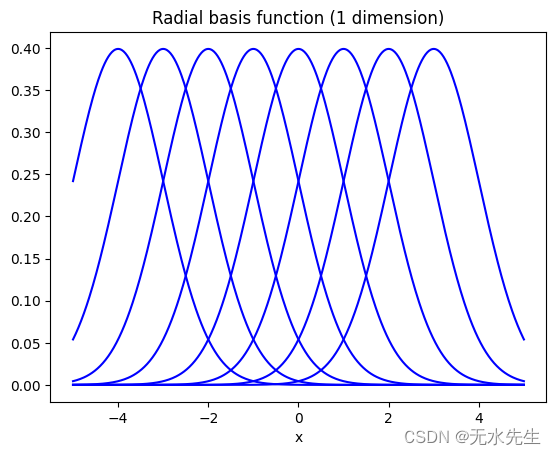
对于基函数,我们可以使用非线性函数,例如多项式项或余弦函数。因此,线性回归模型可以通过将非线性基函数应用于 x 来掌握非线性关系。下图显示了我们使用径向基函数时的示例情况。

具有径向基函数的线性回归模型
如您所见,它可以掌握复杂的数据结构。我们仍然称它为线性回归模型,因为从参数 w 的角度来看,这个方程仍然满足线性关系。您可以检查参数是否没有非线性表达式。
我们也可以用与多元线性回归相同的方式推导参数。以下方程是线性回归模型的矩阵和线性代数形式。我们假设有 N 个数据点和 p+1 参数。
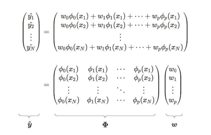
线性回归模型的矩阵形式

线性回归模型的线性代数形式
请注意,矩阵 Φ 值在我们对每个输入数据应用基函数后成为常数。它不是类似于多元线性回归吗?实际上,参数的解析推导是相同的。

线性回归模型与多元线性回归的参数推导
线性回归模型在公式 (4) 中假设一个自变量存在缺陷。因此,当输入数据维度的数量增加时,参数的数量会呈指数增长。如果我们添加基函数的数量,我们可以获得模型的灵活性,但计算量会不切实际地增加。这个问题被称为维度的诅咒。有没有办法在不增加计算量的情况下提高模型的灵活性?是的,我们应用高斯过程定理。让我们进入下一节,看看什么是高斯过程。
四、高斯过程的数学背景
我们已经看到,当参数数量增加时,线性回归模型存在维数诅咒的问题。这个问题的解决方案是对参数进行期望,并创建一个不需要参数来计算的情况。这是什么意思?请记住,线性回归模型公式如下。
线性回归模型的线性代数形式
现在,当我们假设参数 w 遵循高斯分布时,输出 y 将遵循高斯分布,因为矩阵 Φ 只是恒定值矩阵。我们假设该参数遵循下面的高斯分布:

该参数遵循定义的高斯分布
基于此,我们可以按如下方式计算输出分布的参数:
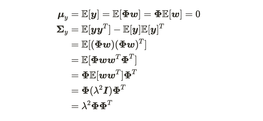
输出分布参数的推导

输出 y 的分布
正如你所看到的,我们可以通过取其期望来抵消参数计算。因此,即使我们有无限的参数,它们也不会影响计算。x 和 y 之间的这种关系遵循高斯过程。高斯过程定义为:

高斯过程的定义
直观地说,高斯过程是具有无限多个参数的多元高斯分布。公式(7)是指给定数据对高斯过程的边际高斯分布。它源于边际多元高斯分布仍然遵循高斯分布的特征。因此,通过充分利用高斯过程,可以在考虑无限维参数的同时构建模型。
这里还有一个问题,我们如何选择矩阵Φ?当我们关注上述公式的协方差矩阵部分并将其设置为 K 时,每个元素可以写成:

公式 (7) 的协方差矩阵
根据公式(9),协方差矩阵的每个元素都是φ(习)和φ(xj)的内积的常数倍数。由于内积类似于余弦相似性,因此当 习 和 xj 相似时,公式 (9) 的值变大。
为了满足协方差矩阵的对称性和正定性且具有逆矩阵的特征,我们需要适当地选择φ(x)。为了实现它们,我们利用 φ(x) 的内核函数。

内核函数
使用核函数的一个好处是,我们可以通过核函数获得 φ(x) 的内积,而无需显式计算 φ(x)。这种技术称为内核技巧。你可以查看这个优秀的博客 [3] 来详细解释内核技巧。最常用的内核函数如下所示。
- 高斯核

高斯核函数
- 线性内核

线性核函数
- 周期性内核

周期性内核
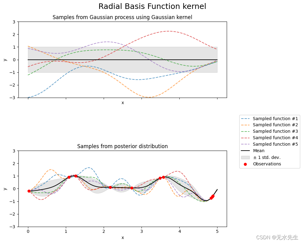
可视化显示了使用每个内核的一维高斯过程的采样。您可以看到内核的功能。
现在,让我们回顾一下高斯过程。使用内核函数,我们可以将定义重写为:

高斯过程的数学定义
当 f 的每个元素都遵循高斯过程(即无限高斯分布)时,f 的联合概率遵循多元高斯分布。
在下一节中,我们将讨论高斯过程或高斯过程回归模型的应用。
五、高斯过程的应用:高斯过程回归
在最后一节中,我们将高斯过程应用于回归。我们将看到下面的主题。
- 如何拟合和推理高斯过程模型
- 示例:一维数据的高斯过程模型
- 示例:多维数据的高斯过程模型
5.1 如何拟合和推理高斯过程模型
让我们有 N 个输入数据 x 和相应的输出 y。

输入数据 x 和相应的输出 y
为简单起见,我们对输入数据 x 进行归一化以进行预处理,这意味着 x 的平均值为 0。如果我们在 x 和 y 之间有以下关系,并且 f 遵循高斯过程。

x 和 y 之间的关系以及高斯过程设置
因此,输出 y 遵循以下多元高斯分布。

高斯过程回归模型
为了拟合,我们只需通过核函数计算协方差矩阵,并将输出 y 分布的参数确定为正好为 1。因此,除了核函数的超参数之外,高斯过程没有训练阶段。
推理阶段怎么样?由于高斯过程没有像线性回归模型那样的权重参数,我们需要再次拟合包括新数据。但是,我们可以使用多元高斯分布的特征来节省计算量。
让我们有 m 个新数据点。
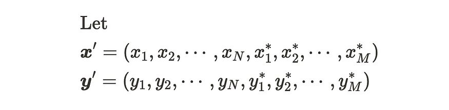
新数据集
在这种情况下,分布(包括新数据点)也遵循高斯分布,因此我们可以将其描述如下:
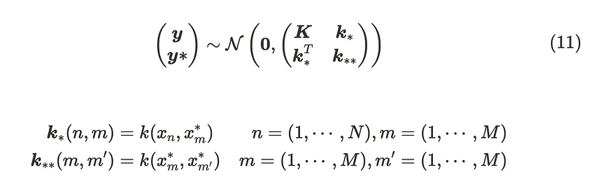
包含新数据点的新发行版
请记住公式(2),条件多元高斯分布的参数。

条件多元高斯分布的参数
当我们将此公式应用于公式 (11) 时,参数如下:

高斯过程回归的更新公式
这是高斯过程回归模型的更新公式。当我们想从中取样时,我们使用从 Cholesky 分解导出的下三角矩阵。
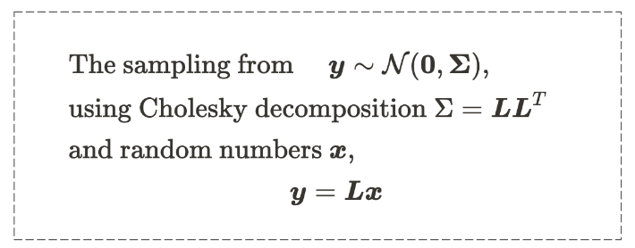
多元高斯分布的采样方法
您可以查看 [4] 中的详细理论解释。但是,在实际情况下,您不需要从头开始实现高斯过程回归,因为 Python 中已经有很好的库。
在下面的小节中,我们将学习如何使用 Gpy 库实现高斯过程。您可以通过 pip 轻松安装它。
5.2 示例:一维数据的高斯过程模型
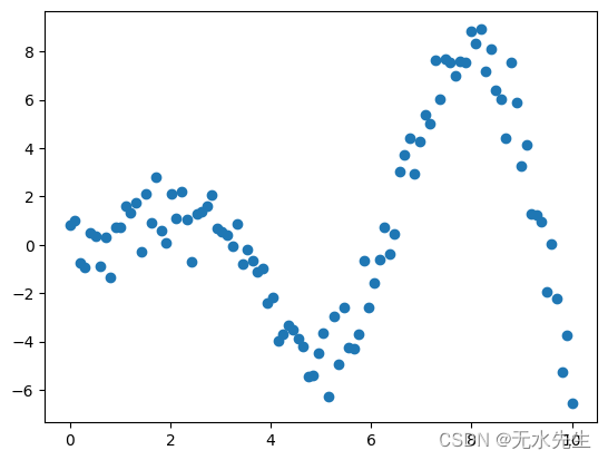
我们将使用一个玩具示例数据,该数据由具有高斯噪声的 sin 函数生成。
# Generate the randomized sample

X = np.linspace(start=0, stop=10, num=100).reshape(-1, 1)
y = np.squeeze(X * np.sin(X)) + np.random.randn(X.shape[0])
y = y.reshape(-1, 1)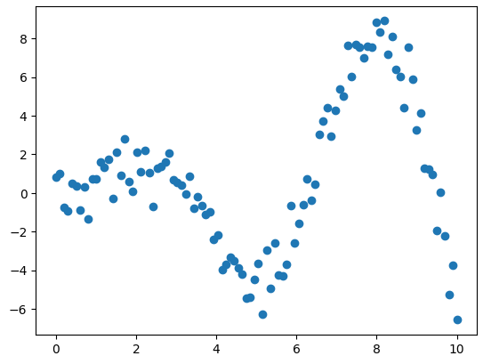
玩具示例
我们使用 RBF 内核是因为它非常灵活且易于使用。多亏了 GPy,我们只需几行即可声明 RBF 核和高斯过程回归模型。
# RBF kernel
kernel = GPy.kern.RBF(input_dim=1, variance=1., lengthscale=1.)

# Gaussian process regression using RBF kernel
m = GPy.models.GPRegression(X, y, kernel)
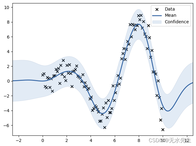
使用高斯过程回归模型的拟合分布
x 点表示输入数据,蓝色曲线表示该点高斯过程回归模型的期望值,浅蓝色阴影区域表示 95% 置信区间。
如您所见,具有多个数据点的区域具有较浅的置信区间,但具有几个点的区域具有较宽的区间。因此,如果你是制造业的工程师,你可以知道你在哪里没有足够的数据,但数据区域(或实验条件)有可能有目标值。
5.3 示例:多维数据的高斯过程模型
我们将使用 scikit-learn 示例数据集中的糖尿病数据集。
# Load the diabetes dataset and create a dataframe
diabetes = datasets.load_diabetes()
df = pd.DataFrame(diabetes.data, columns=diabetes.feature_names)
这个数据集已经过预处理(归一化),所以我们可以直接实现高斯过程回归模型。我们也可以将同一个类用于多个输入。
# dataset
X = df[['age', 'sex', 'bmi', 'bp']].values
y = df[['target']].values

# set kernel
kernel = GPy.kern.RBF(input_dim=4, variance=1.0, lengthscale=1.0, ARD = True)

# create GPR model
m = GPy.models.GPRegression(X, y, kernel = kernel)
结果如下表所示。
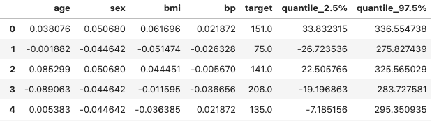
包含输入变量和目标变量的结果表
如您所见,还有很大的改进空间。改进预测结果的最简单步骤是收集更多数据。如果不可能,您可以更改内核的选择或超参数优化。我稍后会粘贴我使用的代码,所以请随意更改和播放它!
您可以使用以下代码重现可视化和 GPy 实验。
我们已经讨论了数学定理和高斯过程的实际实现。当您拥有少量数据时,此技术非常有用。但是,由于计算量取决于数据的数量,请记住它不适合大数据。感谢您的阅读!
六、引用
[1] Mochihashi, D., Oba, S., ガウス過程と機械学習, 講談社
[2]多元正态distribution.pdf的 https://www.khoury.northeastern.edu/home/vip/teach/MLcourse/3_generative_models/lecture_notes/Marginal 分布和条件分布
[3] Hui, J., 机器学习内核, Medium
[4] RPubs - Sampling from Multivariate Normal Random Variable
Mathematical understanding of Gaussian Process | by Yuki Shizuya | The Quantastic Journal | Jun, 2024 | Medium
七、代码参考
import numpy as np
import pandas as pd
import matplotlib.pyplot as plt
from scipy.stats import norm, multivariate_normal
from sklearn.linear_model import LinearRegression
from sklearn import datasets
import GPy
Linear data
In [15]:
n_samples = 30

w0 = 2.0
w1 = 4.5

x = np.sort(np.random.rand(n_samples))
y = w1 * x + w0 + np.random.rand(n_samples)

x = x.reshape(-1, 1)
y = y.reshape(-1, 1)

lr = LinearRegression()
lr.fit(x, y)

print('coefficient:', lr.coef_)
print('intercept:', lr.intercept_)

fig, ax = plt.subplots(1, 2, figsize=(10, 5))

ax[0].scatter(x, y, color='blue', label='input data')
ax[0].set_xlabel('x')
ax[0].set_ylabel('y')

ax[1].scatter(x, y, color='blue', label='input data')
ax[1].plot(x, lr.predict(x), color='black', label='linear regression line')
ax[1].set_xlabel('x')
ax[1].set_ylabel('y')
ax[1].legend()
plt.show()
coefficient: [[4.60793678]]
intercept: [2.38216139]
Non-linear data
In [18]:
n_samples = 30

x = np.sort(np.random.rand(n_samples))
y = np.sin(2.0 * np.pi * x) + np.random.rand(n_samples)

x = x.reshape(-1, 1)
y = y.reshape(-1, 1)

lr = LinearRegression()
lr.fit(x, y)

print('coefficient:', lr.coef_)
print('intercept:', lr.intercept_)

fig, ax = plt.subplots(1, 2, figsize=(10, 5))

ax[0].scatter(x, y, color='blue', label='input data')
ax[0].set_xlabel('x')
ax[0].set_ylabel('y')

ax[1].scatter(x, y, color='blue', label='input data')
ax[1].plot(x, lr.predict(x), color='black', label='linear regression line')
ax[1].set_xlabel('x')
ax[1].set_ylabel('y')
ax[1].legend()

plt.show()
coefficient: [[-2.12667242]]
intercept: [1.5927719]

Radial basis function regression
In [22]:
# the mu values for radial basis function
mus = np.array([i for i in range(-4, 4, 1)])

# 1-D input data
x = np.linspace(-5, 5, 500)

# for visualization
fig, ax = plt.subplots(1, 1)

# calculate the pdf of each mu
for mu in mus:
    rv = norm(loc=mu, scale=1.0)
    ax.plot(x, rv.pdf(x), color='blue')

ax.set_xlabel('x')
ax.set_title('Radial basis function (1 dimension)')
plt.show()
In [33]:
# the mu values for radial basis function
mus = np.array([i for i in range(-4, 5, 1)])

# weights for the spline function
weights = np.array([-0.48, -0.52, 0.1, -0.9, 0.23, 0.57, 0.28, -0.69, 0.46])

# 1-D input data
x = np.linspace(-5, 5, 500)

y = np.zeros(x.shape)

for i in range(len(x)):
    for j in range(len(weights)):
        y[i] += weights[j] * np.exp(-(x[i]-mus[j])**2)

# for visualization
fig, ax = plt.subplots(1, 1)
ax.plot(x, y, color='black')
ax.set_xlabel('x')
ax.set_title('Radial basis function regression')
plt.grid()
plt.show()

Merginal distribution visualization
In [25]:
# Marginal distribution

mus = [[0, 0] for _ in range(3)]
covs = [[[1, 0.2], [0.2, 1]], [[1, 0.5], [0.5, 1]], [[1, 0.8], [0.8, 1]]]

fig, ax = plt.subplots(1, 3, figsize=(15, 5))

max_val = 3
min_val = -3

N = 200
x = np.linspace(min_val, max_val, N)
y = np.linspace(min_val, max_val, N)
X, Y = np.meshgrid(x, y)

pos  = np.dstack((X, Y))

for i in range(3):
    mu = mus[i]
    cov = covs[i]

    rv   = multivariate_normal(mu, cov)
    Z    = rv.pdf(pos)

    ax[i].contour(X, Y, Z)
    ax[i].set_aspect('equal', adjustable='box')

    rv1 = norm(mu[0], cov[0][0])
    z1 = rv1.pdf(x)
    ax[i].plot(x, z1-max_val)

    rv2 = norm(mu[1], cov[1][1])
    z2 = rv2.pdf(y)
    ax[i].plot(z2-max_val, y)

    ax[i].set_xticks([])
    ax[i].set_yticks([])

plt.grid()
plt.show()
Conditional distribution visualization
In [40]:
# Conditional distribution

mus = [0, 0]
covs = [[1, 0.8], [0.8, 1]]

fig, ax = plt.subplots(1, 1)

max_val = 3
min_val = -3

N = 200
x = np.linspace(min_val, max_val, N)
y = np.linspace(min_val, max_val, N)
X, Y = np.meshgrid(x, y)

pos  = np.dstack((X, Y))
rv   = multivariate_normal(mu, cov)
Z    = rv.pdf(pos)

ax.contour(X, Y, Z)
ax.set_aspect('equal', adjustable='box')

for c in [-1.5, 0, 1.5]:
    cond_mu = mu[1] + covs[1][0] * (1 / covs[0][0]) * (c - mu[0])
    cond_cov = covs[1][1] - covs[1][0] * (1 / covs[0][0]) * covs[0][1]

    rv1 = norm(cond_mu, cond_cov)
    z1 = rv1.pdf(x)
    ax.plot(z1+c, x, '--', color='black')
    ax.plot([c for _ in range(len(y))], y, color='black')

plt.grid()
plt.show()
Sampling from Gaussain process using various kernel funcions
In [42]:
import matplotlib.pyplot as plt
import numpy as np


def plot_gpr_samples(gpr_model, n_samples, ax):
    """
    Borrow from https://scikit-learn.org/stable/auto_examples/gaussian_process/plot_gpr_prior_posterior.html

    Plot samples drawn from the Gaussian process model.

    If the Gaussian process model is not trained then the drawn samples are
    drawn from the prior distribution. Otherwise, the samples are drawn from
    the posterior distribution. Be aware that a sample here corresponds to a
    function.

    Parameters
    ----------
    gpr_model : `GaussianProcessRegressor`
        A :class:`~sklearn.gaussian_process.GaussianProcessRegressor` model.
    n_samples : int
        The number of samples to draw from the Gaussian process distribution.
    ax : matplotlib axis
        The matplotlib axis where to plot the samples.
    """

    x = np.linspace(0, 5, 100)
    X = x.reshape(-1, 1)

    y_mean, y_std = gpr_model.predict(X, return_std=True)
    y_samples = gpr_model.sample_y(X, n_samples)

    for idx, single_prior in enumerate(y_samples.T):
        ax.plot(
            x,
            single_prior,
            linestyle="--",
            alpha=0.7,
            label=f"Sampled function #{idx + 1}",
        )
    ax.plot(x, y_mean, color="black", label="Mean")
    ax.fill_between(
        x,
        y_mean - y_std,
        y_mean + y_std,
        alpha=0.1,
        color="black",
        label=r"$\pm$ 1 std. dev.",
    )
    ax.set_xlabel("x")
    ax.set_ylabel("y")
    ax.set_ylim([-3, 3])
Example dataset to visualize sampling values from various kernels
In [56]:
rng = np.random.RandomState(4)
X_train = rng.uniform(0, 5, 10).reshape(-1, 1)
y_train = np.sin((X_train[:, 0] - 2.5) ** 2)
n_samples = 5
In [63]:
from sklearn.gaussian_process import GaussianProcessRegressor
from sklearn.gaussian_process.kernels import RBF, ConstantKernel, DotProduct, ExpSineSquared
In [59]:
# Linear kernel

kernel = (
    ConstantKernel(0.1, (0.01, 10.0)) + DotProduct(sigma_0=0)
)
gpr = GaussianProcessRegressor(kernel=kernel, random_state=0)

fig, axs = plt.subplots(nrows=2, sharex=True, sharey=True, figsize=(10, 8))

# plot prior
plot_gpr_samples(gpr, n_samples=n_samples, ax=axs[0])
axs[0].set_title("Samples from Gaussian process using linear kernel")

# plot posterior
gpr.fit(X_train, y_train)
plot_gpr_samples(gpr, n_samples=n_samples, ax=axs[1])
axs[1].scatter(X_train[:, 0], y_train, color="red", zorder=10, label="Observations")
axs[1].legend(bbox_to_anchor=(1.05, 1.5), loc="upper left")
axs[1].set_title("Samples from posterior distribution")

fig.suptitle("Dot-product kernel", fontsize=18)
plt.tight_layout()
/opt/homebrew/anaconda3/envs/smoothing-env/lib/python3.8/site-packages/sklearn/gaussian_process/kernels.py:284: RuntimeWarning: divide by zero encountered in log
  return np.log(np.hstack(theta))
/opt/homebrew/anaconda3/envs/smoothing-env/lib/python3.8/site-packages/sklearn/gaussian_process/_gpr.py:659: ConvergenceWarning: lbfgs failed to converge (status=2):
ABNORMAL_TERMINATION_IN_LNSRCH.

Increase the number of iterations (max_iter) or scale the data as shown in:
    https://scikit-learn.org/stable/modules/preprocessing.html
  _check_optimize_result("lbfgs", opt_res)
/opt/homebrew/anaconda3/envs/smoothing-env/lib/python3.8/site-packages/sklearn/gaussian_process/kernels.py:419: ConvergenceWarning: The optimal value found for dimension 0 of parameter k2__sigma_0 is close to the specified lower bound 1e-05. Decreasing the bound and calling fit again may find a better value.
  warnings.warn(

In [61]:
# Gaussian kernel

kernel = 1.0 * RBF(length_scale=1.0, length_scale_bounds=(1e-1, 10.0))
gpr = GaussianProcessRegressor(kernel=kernel, random_state=0)

fig, axs = plt.subplots(nrows=2, sharex=True, sharey=True, figsize=(10, 8))

# plot prior
plot_gpr_samples(gpr, n_samples=n_samples, ax=axs[0])
axs[0].set_title("Samples from Gaussian process using Gaussian kernel")

# plot posterior
gpr.fit(X_train, y_train)
plot_gpr_samples(gpr, n_samples=n_samples, ax=axs[1])
axs[1].scatter(X_train[:, 0], y_train, color="red", zorder=10, label="Observations")
axs[1].legend(bbox_to_anchor=(1.05, 1.5), loc="upper left")
axs[1].set_title("Samples from posterior distribution")

fig.suptitle("Radial Basis Function kernel", fontsize=18)
plt.tight_layout()
In [65]:
kernel = 1.0 * ExpSineSquared(
    length_scale=1.0,
    periodicity=1.0,
    length_scale_bounds=(0.1, 10.0),
    periodicity_bounds=(1.0, 10.0),
)
gpr = GaussianProcessRegressor(kernel=kernel, random_state=0)

fig, axs = plt.subplots(nrows=2, sharex=True, sharey=True, figsize=(10, 8))

# plot prior
plot_gpr_samples(gpr, n_samples=n_samples, ax=axs[0])
axs[0].set_title("Samples from Gaussian process using periodic kernel")

# plot posterior
gpr.fit(X_train, y_train)
plot_gpr_samples(gpr, n_samples=n_samples, ax=axs[1])
axs[1].scatter(X_train[:, 0], y_train, color="red", zorder=10, label="Observations")
axs[1].legend(bbox_to_anchor=(1.05, 1.5), loc="upper left")
axs[1].set_title("Samples from posterior distribution")

fig.suptitle("Exp-Sine-Squared kernel", fontsize=18)
plt.tight_layout()
/opt/homebrew/anaconda3/envs/smoothing-env/lib/python3.8/site-packages/sklearn/gaussian_process/kernels.py:429: ConvergenceWarning: The optimal value found for dimension 0 of parameter k2__periodicity is close to the specified upper bound 10.0. Increasing the bound and calling fit again may find a better value.
  warnings.warn(

Example: Gaissian process model for one-dimensional data
The code heavily borrowed from Jupyter Notebook Viewer
In [11]:
# Generate the randomized sample

X = np.linspace(start=0, stop=10, num=100).reshape(-1, 1)
y = np.squeeze(X * np.sin(X)) + np.random.randn(X.shape[0])
y = y.reshape(-1, 1)
In [12]:
# The input data's visualization

plt.scatter(X, y)
plt.show()
In [3]:
# RBF kernel
kernel = GPy.kern.RBF(input_dim=1, variance=1., lengthscale=1.)
In [13]:
# Gaussian process regression using RBF kernel
m = GPy.models.GPRegression(X, y, kernel)
In [14]:
from IPython.display import display
display(m)
Model: GP regression
Objective: 204.66508168561933
Number of Parameters: 3
Number of Optimization Parameters: 3
Updates: True
| GP_regression. | value | constraints | priors |
|---|---|---|---|
| rbf.variance | 1.0 | +ve | |
| rbf.lengthscale | 1.0 | +ve | |
| Gaussian_noise.variance | 1.0 | +ve |
In [15]:
#np.int = np.int32

fig = m.plot()
GPy.plotting.show(fig, filename='basic_gp_regression_notebook')
---------------------------------------------------------------------------
AttributeError                            Traceback (most recent call last)
Cell In[15], line 4
      1 #np.int = np.int32
      3 fig = m.plot()
----> 4 GPy.plotting.show(fig, filename='basic_gp_regression_notebook')

File /opt/homebrew/anaconda3/envs/smoothing-env/lib/python3.8/site-packages/GPy/plotting/__init__.py:150, in show(figure, **kwargs)
    142 def show(figure, **kwargs):
    143     """
    144     Show the specific plotting library figure, returned by
    145     add_to_canvas().
   (...)
    148     for showing/drawing a figure.
    149     """
--> 150     return plotting_library().show_canvas(figure, **kwargs)

File /opt/homebrew/anaconda3/envs/smoothing-env/lib/python3.8/site-packages/GPy/plotting/matplot_dep/plot_definitions.py:96, in MatplotlibPlots.show_canvas(self, ax, **kwargs)
     95 def show_canvas(self, ax, **kwargs):
---> 96     ax.figure.canvas.draw()
     97     return ax.figure

AttributeError: 'dict' object has no attribute 'figure'
In [ ]:
Example : Gaussian process model for multiple dimension data
In [21]:
# Load the diabetes dataset and create a dataframe
diabetes = datasets.load_diabetes()
df = pd.DataFrame(diabetes.data, columns=diabetes.feature_names)
df.head()
Out[21]:
| age | sex | bmi | bp | s1 | s2 | s3 | s4 | s5 | s6 | |
|---|---|---|---|---|---|---|---|---|---|---|
| 0 | 0.038076 | 0.050680 | 0.061696 | 0.021872 | -0.044223 | -0.034821 | -0.043401 | -0.002592 | 0.019907 | -0.017646 |
| 1 | -0.001882 | -0.044642 | -0.051474 | -0.026328 | -0.008449 | -0.019163 | 0.074412 | -0.039493 | -0.068332 | -0.092204 |
| 2 | 0.085299 | 0.050680 | 0.044451 | -0.005670 | -0.045599 | -0.034194 | -0.032356 | -0.002592 | 0.002861 | -0.025930 |
| 3 | -0.089063 | -0.044642 | -0.011595 | -0.036656 | 0.012191 | 0.024991 | -0.036038 | 0.034309 | 0.022688 | -0.009362 |
| 4 | 0.005383 | -0.044642 | -0.036385 | 0.021872 | 0.003935 | 0.015596 | 0.008142 | -0.002592 | -0.031988 | -0.046641 |
In [23]:
# Add the target variable to the dataframe
df['target'] = diabetes.target
In [36]:
# training dataset
X = df[['age', 'sex', 'bmi', 'bp']].values
y = df[['target']].values
In [37]:
# set kernel
kernel = GPy.kern.RBF(input_dim=4, variance=1.0, lengthscale=1.0, ARD = True)
In [38]:
# create GPR model
m = GPy.models.GPRegression(X, y, kernel = kernel, normalizer = True)
In [39]:
display(m)
Model: GP regression
Objective: 580.753895481785
Number of Parameters: 6
Number of Optimization Parameters: 6
Updates: True
| GP_regression. | value | constraints | priors |
|---|---|---|---|
| rbf.variance | 1.0 | +ve | |
| rbf.lengthscale | (4,) | +ve | |
| Gaussian_noise.variance | 1.0 | +ve |
In [46]:
intervals = m.predict_quantiles(X)
In [47]:
df['quantile_2.5%'] = intervals[0]
df['quantile_97.5%'] = intervals[1]
In [48]:
compare_dataset = df[['age', 'sex', 'bmi', 'bp', 'target', 'quantile_2.5%', 'quantile_97.5%']]
In [49]:
compare_dataset.head(20)
Out[49]:
| age | sex | bmi | bp | target | quantile_2.5% | quantile_97.5% | |
|---|---|---|---|---|---|---|---|
| 0 | 0.038076 | 0.050680 | 0.061696 | 0.021872 | 151.0 | 33.832315 | 336.554738 |
| 1 | -0.001882 | -0.044642 | -0.051474 | -0.026328 | 75.0 | -26.723536 | 275.827439 |
| 2 | 0.085299 | 0.050680 | 0.044451 | -0.005670 | 141.0 | 22.505766 | 325.565029 |
| 3 | -0.089063 | -0.044642 | -0.011595 | -0.036656 | 206.0 | -19.196863 | 283.727581 |
| 4 | 0.005383 | -0.044642 | -0.036385 | 0.021872 | 135.0 | -7.185156 | 295.350935 |
| 5 | -0.092695 | -0.044642 | -0.040696 | -0.019442 | 97.0 | -26.981159 | 276.039792 |
| 6 | -0.045472 | 0.050680 | -0.047163 | -0.015999 | 138.0 | -27.454852 | 275.284279 |
| 7 | 0.063504 | 0.050680 | -0.001895 | 0.066629 | 63.0 | 20.998093 | 323.888776 |
| 8 | 0.041708 | 0.050680 | 0.061696 | -0.040099 | 110.0 | 17.424206 | 320.475631 |
| 9 | -0.070900 | -0.044642 | 0.039062 | -0.033213 | 310.0 | 3.966733 | 306.879694 |
| 10 | -0.096328 | -0.044642 | -0.083808 | 0.008101 | 101.0 | -37.940518 | 265.602567 |
| 11 | 0.027178 | 0.050680 | 0.017506 | -0.033213 | 69.0 | 0.072888 | 302.686168 |
| 12 | 0.016281 | -0.044642 | -0.028840 | -0.009113 | 179.0 | -11.453087 | 290.991778 |
| 13 | 0.005383 | 0.050680 | -0.001895 | 0.008101 | 185.0 | 1.531656 | 303.928312 |
| 14 | 0.045341 | -0.044642 | -0.025607 | -0.012556 | 118.0 | -9.027330 | 293.574895 |
| 15 | -0.052738 | 0.050680 | -0.018062 | 0.080401 | 171.0 | 9.386471 | 312.644291 |
| 16 | -0.005515 | -0.044642 | 0.042296 | 0.049415 | 166.0 | 31.992828 | 334.674057 |
| 17 | 0.070769 | 0.050680 | 0.012117 | 0.056301 | 144.0 | 24.619426 | 327.470830 |
| 18 | -0.038207 | -0.044642 | -0.010517 | -0.036656 | 97.0 | -15.012779 | 287.479812 |
| 19 | -0.027310 | -0.044642 | -0.018062 | -0.040099 | 168.0 | -18.277239 | 284.195822 |
In [ ]: